We built an Interactive y⁺ Calculator. Here's Everything It Does.
Near-wall mesh sizing is the single biggest source of silent errors in CFD. This is how we fixed that.
By the Splash-CFD Team · Mesh & Turbulence · 15 min read
Every CFD engineer has been there. You run a simulation, the solver converges, the contours look clean — and then someone asks about y⁺, and the whole thing starts to unravel. Maybe the first cells were sitting in the buffer layer. Maybe the wall function was being applied where the boundary layer was barely developed. The results weren't wrong in an obvious way — they just weren't right in the way that matters.
Near-wall mesh sizing is one of those topics that gets a one-page treatment in textbooks but quietly drives a disproportionate number of simulation errors in practice. Getting y⁺ wrong doesn't crash your solver. It just produces physically incorrect skin friction, drag, heat transfer, and separation prediction — and you only find out when you compare to experimental data you may not have.
We built the Splash-CFD y⁺ Calculator to make this right. It's free, it requires no login, and it goes well beyond a basic cell-height formula. Here's a full breakdown of what it does, how it works, and — more importantly — the physics behind every number it produces.
Table of Contents
What y⁺ actually is
The boundary layer structure you need to memorise
Introducing the Splash-CFD y⁺ Calculator
How the calculator works under the hood
Reading the results correctly
Turbulence model requirements
The five most common y⁺ mistakes
The Law of the Wall, interactively
The OpenFOAM export
What the tool doesn't do
What y⁺ Actually Is
The formal definition is simple enough: y⁺ = y · u_τ / ν. But that equation only becomes useful when you understand what each term is actually doing.
y is the physical distance from the wall to the centre of your first mesh cell. ν is the kinematic viscosity of your fluid. But u_τ — the friction velocity — is the interesting one. It's defined as u_τ = √(τ_w / ρ), where τ_w is the wall shear stress. Friction velocity is essentially a velocity scale constructed from how hard the wall is "gripping" the fluid. It has nothing to do with the bulk flow speed; it's an inner-layer variable that describes the intensity of the turbulent near-wall interaction.
What y⁺ tells you, therefore, is where your first cell sits within the boundary layer structure, normalised by the viscous length scale of that specific flow. A y⁺ of 1 means your first cell centre is one viscous length unit from the wall. A y⁺ of 300 means it's 300 viscous lengths away. The implications for turbulence modelling are completely different in each case.
"Getting y⁺ wrong doesn't crash your solver. It just produces physically incorrect results — and you may not find out until it's too late."
The Boundary Layer Structure You Need to Memorise
The turbulent boundary layer is not uniform. It has a layered structure — each zone governed by different physics — and every turbulence model is calibrated against assumptions about which zone your first cell occupies. Place your cell in the wrong zone and you've violated the model's mathematical foundations from grid generation onwards.
y⁺ Range | Zone | Physics | Compatible Models |
|---|---|---|---|
y⁺ < 5 | Viscous sublayer | Molecular viscosity only. Linear velocity profile: u⁺ = y⁺. Where skin friction originates. | k-ω SST, SA, LES, RSM (required) |
y⁺ 5–30 | Buffer layer | Both molecular and turbulent mechanisms compete. No single law applies. Avoid at all costs. | None reliably. Dead zone. |
y⁺ 30–300 | Log-law region | Turbulent shear dominates. Universal log-law: u⁺ = (1/κ)·ln(y⁺) + B. Wall functions exploit this. | k-ε variants (required), k-ω SST with wall functions |
y⁺ > 300 | Outer layer | Too far from wall. Wall function extrapolation breaks down. Incorrect drag and heat transfer. | Refine. No model works well here. |
The buffer layer — roughly y⁺ 5 to 30 — is the most dangerous zone. Simulations with first cells landing here look fine on the surface. The solver converges, the residuals drop, and the flow field looks plausible. But the physics are wrong because no standard turbulence model formulation is valid in this region. Target y⁺ < 2 for wall-resolved simulations, or y⁺ > 30 for wall function approaches. Everything in between is a problem you're choosing to have.
Introducing the Splash-CFD y⁺ Calculator
The tool is live at splash-cfd.com and requires no account, no signup, and no payment. It runs entirely in the browser.
[Screenshot: Input panel — fluid properties auto-fill from preset, or enter custom values]
The interface splits into three tabs: the calculator itself, a turbulence model reference, and a physics guide with an interactive Law of the Wall chart. You can switch between SI and Imperial units at any point, and there's a Mach number field that flags compressibility effects if your flow goes beyond Ma = 0.3.
Fluid presets cover air at standard and elevated temperature, water at 20°C and 80°C, and engine oil — each with pre-loaded kinematic viscosity and density values. Choose "custom" if you're working with a non-standard fluid or want to override the values directly.
How the Calculator Works Under the Hood
This isn't a lookup table. Every output is computed from the physics of your specific flow condition. The calculation chain goes:
1. Reynolds Number
Re = U∞ · L / ν — straightforward, but it drives everything downstream. The Reynolds number determines where you sit on the turbulent skin friction correlation.
2. Skin Friction Coefficient
This is where geometry matters. The tool uses different correlations depending on what you're simulating:
Flat plate / airfoil (Schlichting):
Cf = 0.058 · Re⁻⁰·²— the turbulent flat plate correlation valid for 5×10⁵ < Re < 10⁷.Pipe / channel (Petukhov):
Cf = (0.790 · ln Re − 1.64)⁻²— the fully-developed internal flow correlation. Gives a meaningfully different result from the flat plate formula at the same Re.
Using the wrong correlation for your geometry can shift your Δy₁ estimate by 30–50%. The tool enforces geometry-appropriate Cf selection — something most online calculators don't bother with.
3. Wall Shear Stress and Friction Velocity
4. First Cell Height from the y⁺ Definition
Rearranging y⁺ = Δy₁ · u_τ / ν for Δy₁:
This is the number that goes directly into your mesh generator.
5. Total Prism Layer Stack
With N layers and growth ratio r, the total prism layer height is the geometric series sum:
The tool also estimates the 99% boundary layer thickness using δ₉₉ ≈ 0.37 · L · Re⁻⁰·² and shows what percentage of δ₉₉ your prism stack covers — a direct indicator of whether your BL is fully captured.
⚠️ Note: These correlations give a pre-simulation estimate based on ideal conditions. After your first run, always inspect wall y⁺ contours. Stagnation points have significantly lower y⁺; separated regions can have much higher y⁺ than the flat-plate estimate predicts.
Reading the Results Correctly
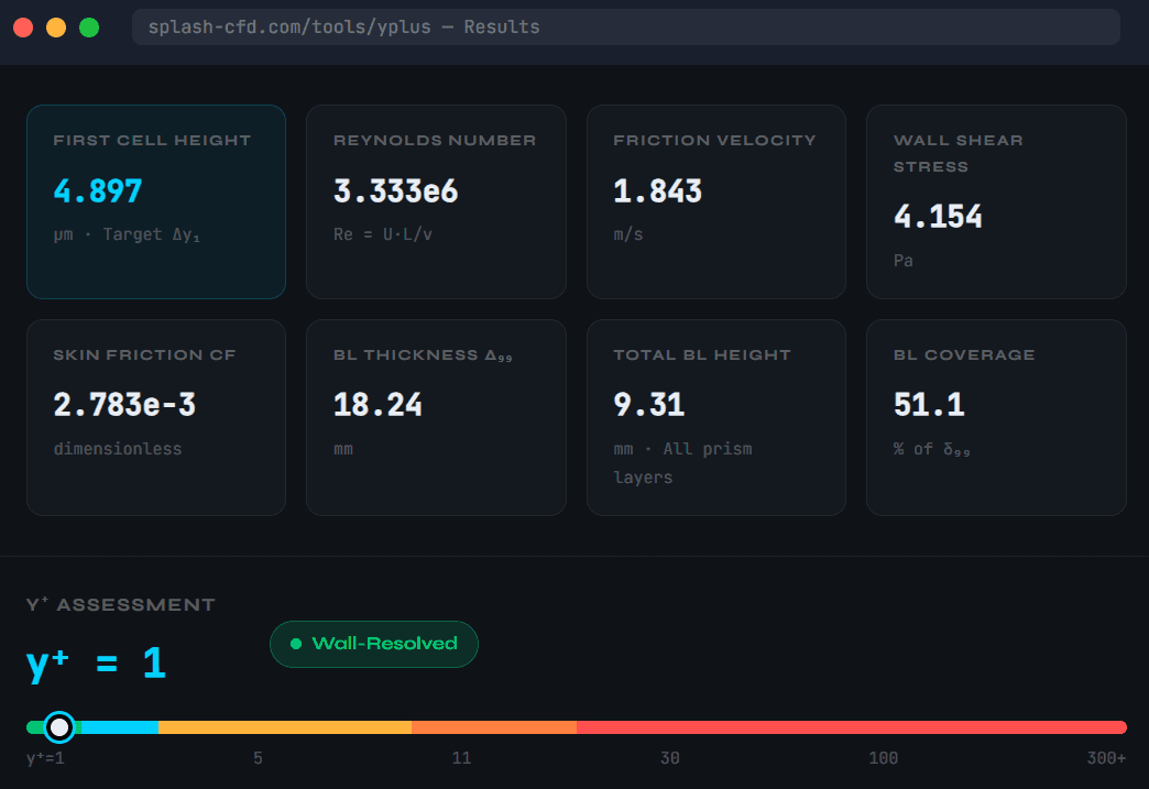
The results are presented as eight computed quantities. The First Cell Height (Δy₁) is the only number most people came for — it goes straight into your mesh generator. But the others matter too.
BL Thickness δ₉₉ and BL Coverage are particularly important and routinely ignored. If your prism stack covers only 40% of the estimated boundary layer, you're leaving the turbulent region partially resolved by isotropic cells — which introduces artificial diffusion and incorrect wall-normal gradients in exactly the region you're trying to capture carefully. A target of 100%+ coverage should be non-negotiable for wall-resolved runs.
The y⁺ gauge at the bottom of the results panel classifies your target into one of five categories — Wall-Resolved, Enhanced Wall Treatment, Buffer Zone (with an explicit caution), Standard Wall Functions, and Too Coarse — with specific advice about which turbulence models are appropriate. The gauge slides smoothly as you adjust inputs, which makes it useful for quick "what if" exploration when you're not yet committed to a specific model.
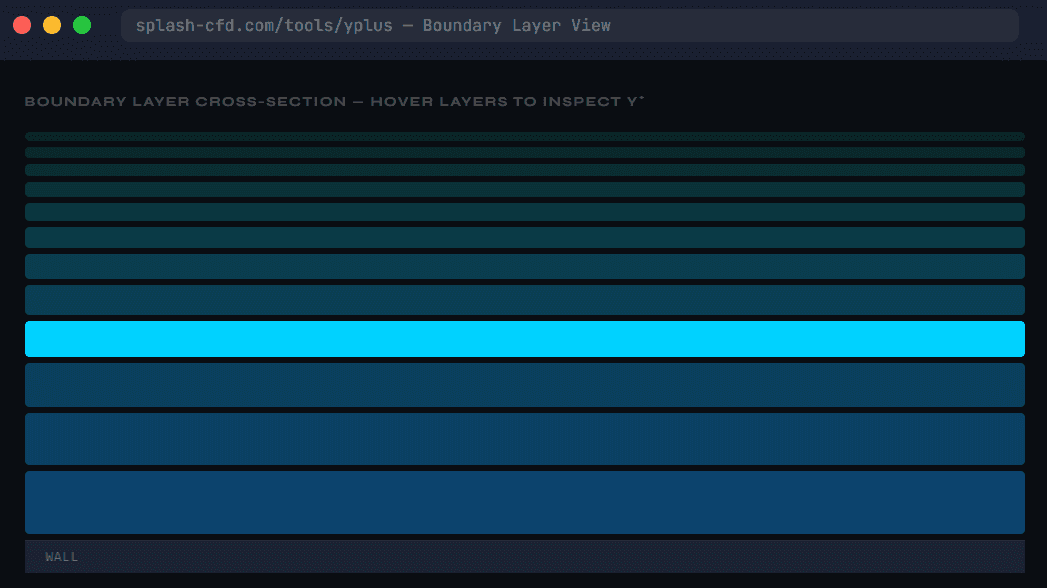
The boundary layer cross-section vew is the part that makes the y⁺ concept visceral rather than abstract. Hover over any prism layer in the stack and the tool computes the local y⁺ at that cell centre, using the actual computed u_τ and your input viscosity. You can immediately see that while your first cell targets y⁺ = 1, by layer 9 or 10 you're already well into the log-law region — which is exactly correct, and is what you want a wall-resolved run to look like.
Turbulence Model Requirements, Explained
The Turbulence Models tab of the tool is a full reference table. But understanding why different models have different y⁺ requirements is more useful than memorising the numbers.
Model | y⁺ Requirement | Treatment | Notes |
|---|---|---|---|
k-ω SST | y⁺ ~ 1 | Low-Re | Industry default for external aero. Integrates directly through viscous sublayer. |
Spalart-Allmaras | y⁺ ~ 1 | Low-Re | One-equation, robust for attached aerospace flows. Unreliable for strong separation. |
k-ε Realizable | y⁺ 30–300 | Wall functions | Best k-ε variant. Better than standard k-ε for separated flows and round jets. |
k-ε Standard | y⁺ 30–300 | Wall functions | Classical model. Avoid for adverse pressure gradients. |
k-ε RNG | y⁺ 30–300 | Wall functions | Better for rotation and swirl. Same y⁺ requirements as standard k-ε. |
RSM | y⁺ ~ 1 | Low-Re | Resolves Reynolds stress anisotropy. Essential for swirling flows and cyclones. High cost. |
LES / DDES | y⁺ ~ 1 | LES | Resolves large eddies directly. Gold standard for unsteady flows. Cost scales steeply with Re. |
WMLES | y⁺ 30–100 | LES + Wall model | Reduces near-wall resolution cost at high Re. Useful compromise for high-Re LES. |
A practical note the tool emphasises: the k-ω SST model is often run with Enhanced Wall Treatment (EWT in Fluent, or nutLowReWallFunction in OpenFOAM), which blends viscous sublayer and log-law formulations using a composite profile. This makes it tolerant of y⁺ values anywhere in the range 1–11 — useful because it's difficult to guarantee y⁺ < 2 everywhere on a complex geometry. Stagnation regions, sharp leading edges, and concave surfaces all create locally elevated u_τ that pulls y⁺ down. If you're using k-ω SST and can't hold y⁺ < 2 everywhere, EWT is your friend.
The Five Most Common y⁺ Mistakes
1. Landing in the Buffer Layer
Targeting y⁺ = 15 is not a compromise between wall-resolved and wall-function approaches. It's a mistake. The buffer layer (y⁺ 5–30) is a region where both viscous and turbulent mechanisms are significant, and no standard turbulence model formulation is accurate here. Choose one side or the other.
2. Insufficient Prism Stack Coverage
Getting the first cell right while terminating the prism layers at 30% of δ₉₉ means you've carefully resolved the viscous sublayer only to have the remaining 70% of the boundary layer captured by isotropic hex or tet cells. This creates a wall-normal gradient discontinuity that corrupts near-wall diffusion. Aim for 100–120% coverage of the estimated δ₉₉.
✅ Rule of thumb: For wall-resolved runs, target at least 10 prism layers covering the full δ₉₉ with a growth ratio ≤ 1.2. The Splash-CFD calculator shows BL coverage percentage directly — aim to keep it above 100%.
3. Growth Ratio Above 1.3
A growth ratio of 1.4 or 1.5 seems harmless — it reduces total cell count and keeps the mesh fast to generate. But above 1.3, the aspect ratio jump between consecutive prism layers introduces interpolation errors at the cell interfaces that contaminate wall-normal gradients. For heat transfer simulations especially, this can produce significant errors even when the first-cell y⁺ is correct.
4. Using the Wrong Cf Correlation
Pipe flow and flat plate flow differ significantly in their skin friction characteristics. At Re = 10⁶, the flat plate Cf is around 0.003 while the pipe Cf is closer to 0.005 — a 60% difference that translates directly into a 60% difference in your Δy₁ estimate. The Splash-CFD tool uses the Petukhov correlation for pipe/channel geometry and Schlichting for external flows, and selects automatically based on your geometry choice.
5. Not Checking y⁺ Post-Simulation
The pre-run estimate is exactly that — an estimate based on a globally-averaged, idealised flow condition. After your first run, inspect wall y⁺ contours on every surface. Pay particular attention to stagnation regions (y⁺ will be much lower than target), sharp features, and separated regions. If large areas of the wall fall outside the intended y⁺ range, you need to locally adapt the mesh before trusting any results.
The Law of the Wall, Interactively
The Physics Guide tab includes an interactive Law of the Wall chart — hover anywhere on it and it reads out u⁺ and y⁺ in real time, along with which zone you're in.
[Screenshot: Interactive Law of the Wall — hover to read u⁺ and y⁺ values with zone identification]
The Law of the Wall is the theoretical backbone of all near-wall turbulence modelling. It states that in the turbulent boundary layer, velocity profiles collapse onto universal curves when normalised by inner variables (u_τ and ν/u_τ). The viscous sublayer obeys u⁺ = y⁺ — a perfectly linear relationship governed entirely by molecular viscosity. The log-law region obeys u⁺ = (1/κ)·ln(y⁺) + B where κ = 0.41 is the von Kármán constant and B ≈ 5.2.
The universality of this curve is what makes wall function approaches possible at all — it means you don't need to resolve the sublayer as long as your first cell sits in a region where the log-law is valid.
The chart also overlays approximate DNS channel flow data, showing how the theoretical curves compare to direct numerical simulation results. The agreement is excellent in the sublayer and log-law regions; in the buffer layer, neither curve is particularly accurate — which is the visual confirmation of why that region is such a problem for modelling.
The OpenFOAM Export
If you're running OpenFOAM, the tool outputs a ready-to-use snappyHexMeshDict block for the addLayersControls section. After you calculate your results, click the OpenFOAM button in the results panel:
The snippet includes the Reynolds number, skin friction coefficient, and friction velocity as comments, so you have a clear record of what the layer sizing was based on. Copy it directly into your case file.
There's also a PDF report download that captures every computed quantity, the full prism layer stack with per-layer heights and y⁺ values, reference equations, and turbulence model recommendations — useful for documenting mesh decisions in a project record or sharing with a team.
What the Tool Doesn't Do (and That's Fine!)
The calculator is an estimation tool, not a mesh generator. It assumes a flat-plate or pipe turbulent boundary layer in equilibrium, which is a reasonable approximation for the pre-mesh-generation phase but will diverge from reality on complex geometries. Strong adverse pressure gradients, laminar-turbulent transition zones, reattachment regions after separation, and three-dimensional effects all produce local y⁺ distributions that differ from the global estimate.
This is expected. The correct workflow is to use the calculator to establish a starting point for Δy₁, build the mesh, run a first-pass simulation, inspect wall y⁺ contours, and iterate. The tool gets you close enough to avoid the most common catastrophic mistakes; post-simulation verification handles the rest.
ℹ️ For compressible flows above Ma = 0.3, the tool flags a warning and recommends applying the van Driest transformation to the skin friction correlation. Standard incompressible Cf can overestimate Δy₁ by 5–20% in transonic conditions.
The tool is free and it stays free. Head to splash-cfd.com to try it. If you have feedback — missing fluid types, additional correlations you'd like to see, questions about specific turbulence model behaviour — reach out via the site. We build these tools because getting near-wall mesh sizing right is genuinely hard, and it shouldn't require a CFD textbook on your desk every time you start a new case.
© 2026 Splash-CFD · splash-cfd.com · Built for engineers who care about getting the physics right.